次のページ
目次
ホームページ
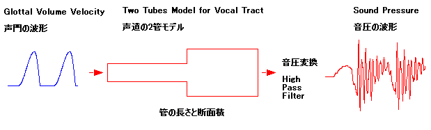
その1: 声門波形と2管声道モデルによる音
声波形の生成 と 数値計算ソフトのSCILABプログラム
人間の声の発生の過程を単純化した模型をつかって、
音声の波形の生成を理解してみよう。
声の発生は、まず、のどの下にある声門で声帯が振動することで、下図の左側の青色のような形の波形が発生する。そして、声帯から喉そして口の中から唇まで
の間を下図の真中のように2つの管(チューブ)がつなぎ合わさった物で置き換えてみる。先ほどの青色の波形がこの2つの管に入力されるとある特定の音の組
み合わせで共鳴しよく響く。そして、口から出てくる空気の流れ、つまり音声を、音圧を検出するマイクで音を拾うと、下図の右側の赤色のような波形になる。
実際の声門の波形はもっと複雑だし、声帯から喉そして口の中から唇までは途中曲がっていて歯も舌も鼻もあるのに、たった2つの管(チューブ)のつなぎ合わ
せで置き換えるのはちょっと
飛躍しすぎている感があるが、こんな簡単化した模型でも、何となく「あ」とか「え」とか聞こえるのである。「あ」
の音(発音記号の/a/)と、「え」の音(発音記号の/ae/)と、「う(い)」の音(発音記号の/ui/)の.wavサンプルをリンクしておこう。この2つの管(チューブ)のつな
ぎ合わせた模型で生成できるのは、「あ」と「え」と「う」の3つの音に限られる。 (「お」については
こちら。 また、「い」についてはこちら。 子音についてはこちら。)
この模型では、主に、2つの管(チューブ)の長さと断面積を変化させて、「あ」とか「え」などの音の調整を行う。管(チューブ)と言っても想像がつかない
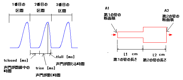
かもしれないが、例えば、水道管、ガス管、または車やバイクについているマフラーも長い管である。下の右側の図は、長さがL1 cmで断面積がA1 cm2の
管に、長さがL2 cmで断面積がA2 cm2の管をつなぎ合わせたイメージ図を示している。このつなぎ合わせた第1の管の左側
(声門側に相当)から、声門からの空気の流れが入ると、2つの管でその長さ分の流れの遅延が生じる、また、断面積の違う2つの管のつなぎ目で音が反射す
る、その結果、いろいろな音の共鳴が起きる。そして、第2の管の右側(口または唇に相当)から出て行く。
入力となる声門の波形は、声門が閉鎖しているとき、声門が開くとき(つまり肺からの空気が出てくるとき)、また、声門が閉じるとき(肺からの空気の流れが
止めようとするとき)、の3つの時間を可変できる。この3つの時間を足し合わせたもの(1区間)が、音の高さを決める、いわゆるピッチ周期に相当する。
ピッチ周期が短いと高い音に聞こえ、ピッチ周期が長いと低い音(低音)に聞こえる。そして、声門の閉鎖そして開いて閉じるを繰り返して、下図の左側の青色
のように山の形が幾つか続く波形となる。
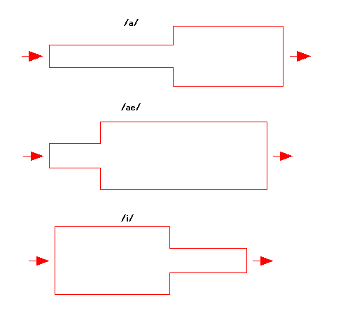
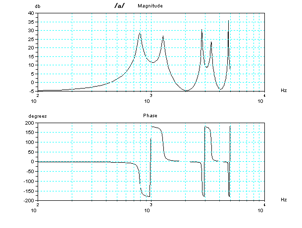
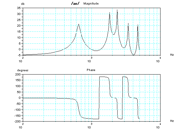
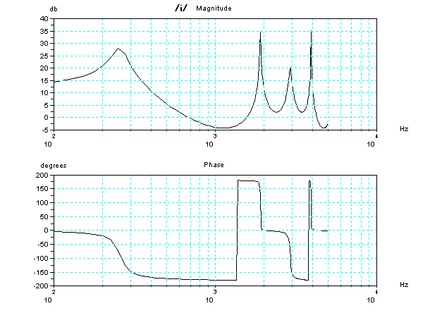
「あ」の音(発音記号の/a/)と「え」の音(発音記号の/ae/)と「い」の音(発音記号の/i/)を生成するための2管(チューブ)の例として
は、下記の形状のような寸法がある。(後述する理由で「い」の音は「う」に近い音になっている。) これが唯一の寸法と言うわけではなく、多の
中のひとつの例である。
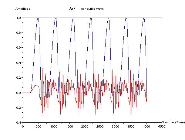
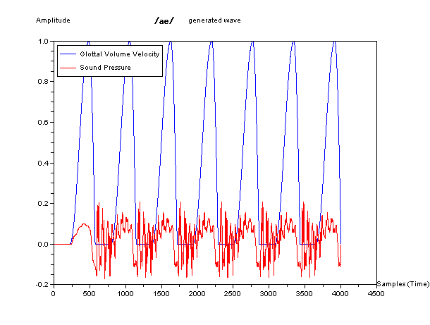
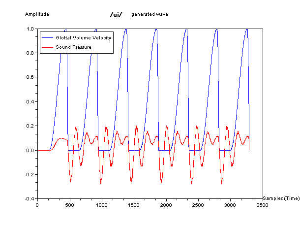
そして、下図が、この単純化した模型で生成した波形の例である。青色が声門の波形を、赤色が音声に相当する音圧の波形をしめしている。
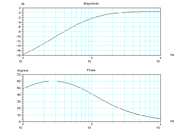
ちょっと専門的な内容になるが、それぞれの、2管声道モデルの周波数と位相の特性(ボード線図)を参考にのせておこう。周波数にピークがある特定の音の組
み合わせが共鳴する可能性がある。但し、共鳴するためには、その周波数の成分が入力されることが条件である。共鳴する可能性があっても、入力にその成分が
欠けていると、無いのと同じである。一番下の「い」の音(発音記号の/i/)は、「う」の音に更に およそ2KHz以上とかの高い周波数の帯域の成分があ
るこ
と
が
特徴であるが、残念ながらこの単純化した模型では、2KHz以上の高い周波数の帯域が欠けているので、「う」に近い音に聞こえてしまうのである。声門の波
形の
変化をより急進に鋭くして、入力である
声門の波形の2KHz以上の高い周波数の帯域の成分をおおく含むようにしてはいるのであるが、まだ、不十分な状態だ。ここでは2KHzと書いたが、実際に
は、発声する人によって周波数とその帯域の値はちがってくる。
また、「お」を生成するためいは、2
つの管(チューブ)では足りない。3つの管(チューブ)による「お」の生成のこころみを別のページにの
せておこう。また、ノイズもつかって生成する「い」についてはこちらのページを見てほしい。
参考までに、管による声道モデルを計算するpythonプログラムをおいておきます。使い方は解凍してできるdocsディレクトリの中のindex.htmlを見てください。
また、フランス発の数値演算ライブラリ
SCILAB を使って、この擬似的に人の音声のような波形を生成するサンプルプログラムを作ってみたので紹介しよう。
声門波形と2管声道モデルによる音声波形の生成のサンプルプログラム TubeModel22.sciを以下に示す。
このサンプルを実際に動作させるためには、
ご使用されるプログラミング環境に合わせて修正・変更・追加などが必要かもしれません。
また、バグが含まれている可能性があります。
万一、このサンプルを動作させる場合は、あなたの責任でおこなってくださいね。
//---------------------------------------------------------------------------
// Two Tubes Model for Vocal Tract
//
.........................................................................................
// PLEASE PAY ATTENSION that this program may have some bugs and also
you may modify program
// to fit your circumstances. If you use this program, everything done
by your own risk.
// Thanks.
//~~~~~~~~~~~~~~~~~~~~~~~~~~~~~~~~~~~~~~~~~~~~~~~~~~~~~~~~~~~~~~~~~~~~~~~~~~~~~~~~~~~~~~~~~~
// Physical Parameters (length and area) Setup
D_QTY=7;
// set dimension of list. This defines length of generated wave
// Generated wave's length will be around D_QTY * (N1+N2+N3).
// sample length & area for /a/ from problems 3.8 in Digital
Processing of Speech Signals by L.R.Rabiner and R.W.Schafer
L1=[9, 9, 9, 9, 9, 9, 9]; // set list of 1st
tube's length by unit is [cm]
A1=[1, 1, 1, 1, 1, 1, 1]; // set list of
1st tube's area by unit is [cm^2]
L2=[8, 8, 8, 8, 8, 8, 8]; // set list of 2nd
tube's length by unit is [cm]
A2=[7, 7, 7, 7, 7, 7, 7]; // set list of
2nd tube's area by unit is [cm^2]
// sample length & area for /ae/ from problems 3.8 in Digital
Processing of Speech Signals by L.R.Rabiner and R.W.Schafer
//L1=[4, 4, 4, 4, 4, 4, 4]; // set list of 1st
tube's length by unit is [cm]
//A1=[1, 1, 1, 1, 1, 1, 1]; // set list
of 1st tube's area by unit is [cm^2]
//L2=[13, 13, 13, 13, 13, 13, 13]; // set list
of 2nd tube's length by unit is [cm]
//A2=[8, 8, 8, 8, 8, 8, 8]; // set list
of 2nd tube's area by unit is [cm^2]
// sample length & area for /i/ from problems 3.8 in Digital
Processing of Speech Signals by L.R.Rabiner and R.W.Schafer
//L1=[9, 9, 9, 9, 9, 9, 9]; // set list of 1st
tube's length by unit is [cm]
//A1=[8, 8, 8, 8, 8, 8, 8]; // set list
of 1st tube's area by unit is [cm^2]
//L2=[6, 6, 6, 6, 6, 6, 6]; // set list of 2nd
tube's length by unit is [cm]
//A2=[1, 1, 1, 1, 1, 1, 1]; // set list
of 2nd tube's area by unit is [cm^2]
c0=35000; // constant. the speed of sound is round
35000 cm/second
tu1=L1./c0; // delay time in 1st tube
tu2=L2./c0; // delay time in 2nd tube
r1=(A2-A1)./(A2+A1); // reflection coefficient between 1st tube
and 2nd tube
//---------------------------------------------------------------------------
// Input Glottal Volume Velocity for Two Tubes Model for Vocal Tract
// A.E.Rosenberg's formula as Glottal Volume Velocity
// Physical Parameters (duration) Setup
//
//D_QTY // set
dimension of list. This defines length of generated wave
tclosed=[5, 5, 5, 5, 5, 5, 5] ; // set
glottis closed duration (off time) by unit is millisecond [ms]
trise= [6, 6, 6, 6, 6, 6, 6]; // set
glottis opening duration (rise time) by unit is millisecond [ms]
tfall= [2, 2, 2, 2, 2, 2, 2]; // set glottis closing duration
(fall time) by unit is millisecond [ms]
// below (tfall is smaller) is for /i/ that needs higher
frequency signals as input
//tclosed=[4, 4, 4, 4, 4, 4, 4] ; // set
glottis closed duration (off time) by unit is millisecond [ms]
//trise= [6, 6, 6, 6, 6, 6, 6]; // set
glottis opening duration (rise time) by unit is millisecond [ms]
//tfall= [0.7, 0.7, 0.7, 0.7, 0.7, 0.7, 0.7]; // set glottis
closing duration (fall time) by unit is millisecond [ms]
amplitude=[1, 1, 1, 1, 1, 1, 1]; // set value of multiplier
// reflection coefficient between glottis and 1st tube
rg_rise=0.9; // set some value (1. or less)
when glottis is opening
rg_fall=0.95; // set some value (1. or less) when
glottis is closing
rg_closed=1; // When glottis is closed,
// reflection coefficient between glottis and 1st tube is 1
// because glottis's gate is closed and vocal tract is free from
glottis's influence
//---------------------------------------------------------------------------
// Output Sound Pressure for Two Tubes Model for Vocal Tract
// Convert from Volume Velocity to Sound Pressure using High Pass
Filter Model for Mouth Radiation
// Parameters ( cut off frequecny ) Setup
//
fc=1000; // set cut off frequency of High Pass Filter by
unit is [Hz]
fnew=fc;
// reflection coefficient between 2nd tube and mouth
rl=0.9; // set adjust reduction response. rl is variable,
however use one constant in this.
//---------------------------------------------------------------------------
// Other preparation: Sampling Frequency Setup
//
fs=44100; // set sampling frequency by unit is [Hz]
ts=1/fs;
//
//==========================================================================
//
// Step 1 Input Glottal Volume Velocity Generation
//
mess1='+++enter step 1 Input Glottal Volume Velocity Generation';
mess1
// length0 is wave length
length0=0;
N1= zeros(1, D_QTY);
N2= zeros(1, D_QTY);
N3= zeros(1, D_QTY);
for loop=1:D_QTY
N1(loop)= int( tclosed(loop) / 1000 / ts );
N2(loop)= int( trise(loop) / 1000 / ts);
N3(loop)= int( tfall(loop) / 1000 / ts);
LL(loop)= N1(loop)+N2(loop)+N3(loop);
length0 = length0 + LL(loop);
end
// yg is Glottal Volume Velocity. rg is reflection coefficient
between glottis and 1st tube
yg= zeros(1,length0+1);
rg= zeros(1,length0+1);
tc0=1;
yg(tc0)=0.;
yg(tc0)=amplitude(1) * yg(tc0);
for loop=1:D_QTY
for t0=1:int(LL(loop))
tc0=tc0+1;
if t0 < N1(loop) then
yg(tc0) =0;
rg(tc0)=rg_closed;
elseif t0 <= (N2(loop) + N1(loop)) then
yg(tc0)= 0.5 * ( 1 - cos( ( %pi / N2(loop) ) * (t0 -
N1(loop)) ) );
rg(tc0)=rg_rise;
elseif t0 <= (N3(loop)+N2(loop)+N1(loop)) then
yg(tc0)= cos( ( %pi / ( 2 * N3(loop) )) * ( t0 -
(N2(loop)+N1(loop)) ) );
rg(tc0)=rg_fall;
else
yg(tc0) =0;
rg(tc0)=rg_closed;
end
yg(tc0)=amplitude(loop) * yg(tc0);
end // t0
end // loop
// function save yg (Glottal Volume Velocity) as one sound wave file
function save_as_sound_file_yg( filename)
max01=0.;
for loop=1:length0
if abs( yg(loop) ) > max01 then
max01 = abs( yg(loop));
end
end
y3out2=zeros(1,length0+1)';
if max01 > 0. then
for loop=1:length0
y3out2(loop)= yg(loop) / max01;
end
end
wavwrite(y3out2, fs, 16, filename );
endfunction
// Function for yg (Glottal Volume Velocity) frequency-phase response
function yg_bode(ni)
frq=[100:25:5000];
frqs=size(frq);
resp=zeros(1,frqs(2));
stp=0;
if ni > 1 then
for v=1:(ni-1)
stp=stp + LL(v);
end
end
stp=stp+N1(ni);
y00=0.;
for v=1:(N2(ni)+N3(ni)+1)
y00= y00 + yg(stp + v);
end
for w=1:frqs(2)
xw=2 * %pi * frq(w) * ts;
yi=0;
for v=1:(N2(ni)+N3(ni)+1)
yi= yi + yg(stp + v) * %e^(-1. * xw * (v-1) * %i);
end // for v
resp(w)=yi / y00;
end // for w
[db,phi] =dbphi(resp);
clf();
bode(frq,db,phi);
endfunction
//
// End of Step 1 Input Glottal Volume Velocity Generation
//
//==========================================================================
//
// Step 2 Two Tubes Model for Vocal Tract Calculation
//
mess2='+++enter step 2 Two Tubes Model for Vocal Tract
Calculation';
mess2
// yt is output of Two Tubes Model for Vocal Tract
M1= zeros(1, D_QTY);
M2= zeros(1, D_QTY);
y2tm= zeros(1,length0+1);
for loop=1:D_QTY
M1(loop)= int( tu1(loop) / ts ) + 1;
M2(loop)= int( tu2(loop) / ts ) + 1;
end
MAX_M1=M1(1);
MAX_M2=M2(1);
for loop=1:D_QTY
if M1(loop) > MAX_M1 then
MAX_M1= M1(loop)
end
if M2(loop) > MAX_M2 then
MAX_M2= M2(loop)
end
end
ya1= zeros(1,MAX_M1);
ya2= zeros(1,MAX_M1);
yb1= zeros(1,MAX_M2);
yb2= zeros(1,MAX_M2);
tc0=1;
ya1(tc0)=0.;
ya2(tc0)=0.;
yb1(tc0)=0.;
yb2(tc0)=0.;
y2tm(tc0)=0.;
for loop=1:D_QTY
for t0=1:int(LL(loop))
tc0=tc0+1;
for jl=MAX_M1:-1:2
ya1(jl)=ya1(jl-1);
ya2(jl)=ya2(jl-1);
end
for jl=MAX_M2:-1:2
yb1(jl)=yb1(jl-1);
yb2(jl)=yb2(jl-1);
end
ya1(1)= ((1. + rg(tc0) ) / 2.) * yg(tc0) + rg(tc0) *
ya2(M1(loop));
ya2(1)= -1. * r1(loop) * ya1(M1(loop)) + ( 1. -
r1(loop) ) * yb2(M2(loop));
yb1(1)= ( 1 + r1(loop) ) * ya1(M1(loop)) + r1(loop) *
yb2(M2(loop));
yb2(1)= -1. * rl * yb1(M2(loop));
y2tm(tc0)= (1 + rl) * yb1(M2(loop));
end // t0
end //loop
// Function for disply two tubes model's frequency-phase response when
glottis is closed
function y = two_tubes( xw, ni, rg0, rl0 )
yi = 0.5 * ( 1 + rg0 ) * ( 1 + r1(ni)) * ( 1 +
rl0 ) * %e^( -1 * ( tu1(ni)
+ tu2(ni) ) .* xw * %i);
yb = 1 + r1(ni) * rg0 * %e^( -2 * tu1(ni) .* xw * %i) +
r1(ni) * rl0 * %e^( -2 * tu2(ni) .* xw * %i) + rl0 * rg0 * %e^( -2 *
(tu1(ni) + tu2(ni)) .* xw * %i);
y = yi ./ yb;
endfunction
function two_tubes_model_bode(ni)
frq=[100:25:5000]';
[db,phi] =dbphi(two_tubes(2 * %pi * frq, ni,rg_closed ,rl));
clf();
bode(frq,db,phi);
endfunction
// Function plot sqrt(area) vs length
function plot_area(ni)
clf();
plot2d(0,0,1,"010","",[-5,-10,20,10],[5,5,4,5]);
ya1=sqrt(A1(ni) );
ya2=sqrt(A2(ni) );
xp=[0 0 L1(ni)
L1(ni) L1(ni)+L2(ni) L1(ni)+L2(ni)
L1(ni) L1(ni) 0 ]';
yp=[ya1 -ya1 -ya1
-ya2
-ya2
ya2
ya2 ya1 ya1 ]';
xpolys( xp, yp, [5 5 5 5 5 5 5 5] );
xar=[-2 -0.5];
yar=[0 0];
xarrows(xar, yar, 1, 5);
xar=[ L1(ni)+L2(ni)+0.5 L1(ni)+L2(ni)+2];
xarrows(xar, yar, 1, 5);
endfunction
//
// End of Step 2 Two Tubes Model for Vocal Tract Calculation
//
//==========================================================================
//
// Step 3 Output Sound Pressure for Two Tubes Model for
Vocal Tract Calculation
//
mess3='+++enter step 3 Output Sound Pressure for Two Tubes Model
for Vocal Tract Calculation';
mess3
// At first, low pass filter's coefficients
wc=2. * %pi * fc;
al1= -1. * %e^( -1. * wc * ts);
bl0= wc * ts;
// Then, convert them to high pass filter's coefficients
function y=f_alfa( wc_org, wc_new)
y= -1. * cos( (wc_org + wc_new) * ts /2. ) / cos( (wc_org -
wc_new) * ts / 2. );
endfunction
wnew=2. * %pi * fnew;
alfa=f_alfa( wc, wnew );
// high pass filter's coefficients
bh0= bl0 / (1.0 - al1 * alfa);
bh1= alfa * bl0 / (1.0 - al1 * alfa);
ah1= (alfa - al1) / (1.0 - al1 * alfa);
// IIR type high pass filter
y3out= zeros(1,length0+1);
LI1=2;
LI2=2;
ya1= zeros(1,LI1);
yb1= zeros(1,LI2);
//loop
for loop=1:length0
ya1(LI1)=ya1(1);
yb1(LI2)=yb1(1);
ya1(1)=y2tm(loop);
yb1(1)= bh0 * ya1(1) + bh1 * ya1(LI1) - ah1 * yb1(LI2);
y3out(loop)=yb1(1);
end //loop
// Function for disply high pass filter's frequency-phase response
function y = hpf1( xw )
yi= bh0 + bh1 * cos( xw * ts) - bh1 * sin( xw * ts ) * %i;
yb=1.0 + ah1 * cos( xw * ts ) - ah1 * sin( xw *
ts ) * %i;
y=yi ./yb;
endfunction
function hpf_bode()
frq=[100:25:10000]';
[db,phi] =dbphi(hpf1(2 * %pi * frq ));
clf();
bode(frq,db,phi);
endfunction
// function save y3out (Sound Pressure) as one sound wave file
function save_as_sound_file( filename)
max01=0.;
for loop=1:length0
if abs( y3out(loop) ) > max01 then
max01 = abs( y3out(loop));
end
end
y3out2=zeros(1,length0+1)';
if max01 > 0. then
for loop=1:length0
y3out2(loop)= y3out(loop) / max01;
end
end
wavwrite(y3out2, fs, 16, filename );
endfunction
//
//
// End of Step 3 Output Sound Pressure for Two Tubes Model
for Vocal Tract
//
//================================================================================
//
// Step 4 Plot Glottal Volume Velocity and Sound Pressure
//
mess4='+++enter step 4 Plot generated sound wave';
mess4
clf();
plot(yg,'b');
plot(y3out,'r');
xtitle('generated wave','Samples (Time)', 'Amplitude');
legend('Glottal Volume Velocity','Sound Pressure',2);
//
//================================================================================
//
// other functions
//
//yg_bode(1) // plot yg (Glottal Volume Velocity)
frequency-phase response
//two_tubes_model_bode(1) // plot Two Tubes Model's
frequency-phase response
//hpf_bode() // plot high pass filter's
frequency-phase response
//save_as_sound_file_yg( 'yg.wav' ) // save yg (Glottal Volume
Velocity) as one .wav file
//save_as_sound_file( 'y3out.wav' ) // save y3out (Sound
Pressure) as one .wav file
//plot_area(1) // plot sqrt(area) vs length
以上が サンプルプログラム TubeModel22.sci である。SCILABの古いバージョンであるがwindows用のscilab-
3.1.1
をつかって動作確認している。 scilab- 4.1.2 向けのプログラムはこちら、また
は、 音をまとめて生成するサンプルプログラム。
注意事項。SCILABもバージョンによって仕様が違い上手く動かない箇所がある。例えば、さらに古いバージョンでは、波形を描
くためにつかっている plot
で、線の属性(実線とか破線とか、また、色など)を定義できないので、線の色などを別に定義するようにplotを変更し設定を追加する必要がある。
windows用のscilab-4.1.2では、波形を.wavでファイルに書き出す wavwrite
の仕様が変更(多チャンネル化対応?)されているため、このままだと、サウンドプレーヤーで再生できない。これを回避するためには、wavwrite
の引数の波形データの形式を 列 から 行 に変更する必要がある。 また、windows用のscilab-4.1.2では、矢印を描く
xarrows の矢印の大きさの定義もかわっている。そこで、断面積を描くなかで使用している
xarrows の矢印の大きさの数を大きく変更しないと、矢印ではなくただの横線になってしまう。
また、設定可能なパラメーターの内容は
区間の数を記入する。これで作る波形の長さを設定する。
D_QTY=7;
// set dimension of list. This defines length of generated wave
// Generated wave's length will be around D_QTY * (N1+N2+N3).
L1が第1管の長さで、A1が断面積、L2が第2管の長さで、A2が断面積。それぞれの区間の値を記入する。
// sample length & area for /a/ from problems 3.8 in Digital
Processing of Speech Signals by L.R.Rabiner and R.W.Schafer
L1=[9, 9, 9, 9, 9, 9, 9]; // set list of 1st
tube's length by unit is [cm]
A1=[1, 1, 1, 1, 1, 1, 1]; // set list of
1st tube's area by unit is [cm^2]
L2=[8, 8, 8, 8, 8, 8, 8]; // set list of 2nd
tube's length by unit is [cm]
A2=[7, 7, 7, 7, 7, 7, 7]; // set list of
2nd tube's area by unit is [cm^2]
声門の波形の各区間の、声門閉鎖時間、声門開く時間、声門閉じる時間を記入する。
tclosed=[5, 5, 5, 5, 5, 5, 5] ; // set
glottis closed duration (off time) by unit is millisecond [ms]
trise= [6, 6, 6, 6, 6, 6, 6]; // set
glottis opening duration (rise time) by unit is millisecond [ms]
tfall= [2, 2, 2, 2, 2, 2, 2]; // set glottis closing duration
(fall time) by unit is millisecond [ms]
声門の波形の各区間の振幅の大きさを記入する。
amplitude=[1, 1, 1, 1, 1, 1, 1]; // set value of multiplier
声門と第1管との反射係数。声門開く、声門閉じる、声門閉鎖のそれぞれを、各区間記入する。
// reflection coefficient between glottis and 1st tube
rg_rise=0.9; // set some value (1. or less)
when glottis is opening
rg_fall=0.95; // set some value (1. or less) when
glottis is closing
rg_closed=1; // When glottis is closed,
// reflection coefficient between glottis and 1st tube is 1
// because glottis's gate is closed and vocal tract is free from
glottis's influence
音圧変換に使っている、IIR型のハイパスフィルターのカットオフ周波数を設定する。
声門開閉時に生じる音圧の波形のバウンドの状態を調整できる。
fc=1000; // set cut off frequency of High Pass Filter by
unit is [Hz]
第2管と外側(口に相当)での反射係数。 音圧の波形の振動の減衰度合いを調整することができる。
// reflection coefficient between 2nd tube and mouth
rl=0.9; // set adjust reduction response. rl is variable,
however use one constant in this.
サンプリング周波数を設定する。音速35000cm/secで1cm進む時間は、サンプリング周波数44.1KHzのときに1.26サンプルである。
管の長さの計算上の分解能をあげるにはサンプリング周波数をもっと高くすることが必要である。
fs=44100; // set sampling frequency by unit is [Hz]
その他、補助的につかえる関数は、
other functions
声門の波形のボード線図(周波数と位相)を描く関数。
yg_bode(1) // plot yg (Glottal Volume Velocity)
frequency-phase response
2管モデルのボード線図(周波数と位相)を描く関数。
two_tubes_model_bode(1) // plot Two Tubes Model's
frequency-phase response
音圧変換に使用しているハイパスフィルターのボード線図(周波数と位相)を描く関数。
hpf_bode() // plot high pass filter's
frequency-phase response
声門の波形を .wav ファイルとして保存する関数。
save_as_sound_file_yg( 'yg.wav' ) // save yg (Glottal Volume
Velocity) as one .wav file
音圧の波形を .wav ファイルとして保存する関数。
save_as_sound_file( 'y3out.wav' ) // save y3out (Sound
Pressure) as one .wav file
2管モデルの管の長さと断面積を描く関数。
plot_area(1) // plot sqrt(area) vs length
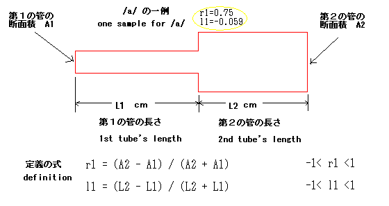
番外: 「あ」(発音記号/a/)の2管
(チューブ)の模型における位置
2管声道モデルで作成した「あ」(発音記号の/a/)が、2管(チューブ)の模型を使って生成される波形の世界の中で、どの位置にあるかを見て
みよう。 このページの前の方でふれた「あ」(発音記号の/a/)の例は下図に示される長さと断面積をもつ2つの管(チューブ)を組み合わせたものであっ
た。
2管(チューブ)の模型で生成される波形の世界を考えるため、上図の様に定義される r1 と l1 の2つのパラメーターを考えてみよう。r1は、2つ
の管(チューブ)の断面積の関係をあらわすもので、ラッパに例えると、r1の値が1に近いほど先端が大きく開いていることを意味する。逆に、r1が-1に
近いほど、先が閉じている。また、l1は、2つの管の長さの関係を示すもので、l1が0であると、2つの管の長さは同じとなる。
この「あ」(発音記号の/a/)の一例では、r1が 0.75で先が開きぎみで、 l1が
-0.059でほぼ管の長さは同じとなっている。
先が閉じているより、拡声器のように、先が開いている方が、つまり、r1が1に近い方が、音量が大きくな
ることが予想されるであろう。また、管の長さが同じとき、つまり、l1がだいたい0のときは、2管(チューブ)の中の共鳴で生じた大きな2つの波の、振動
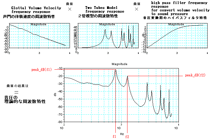
数がいちばん近づくのである。これを見るため、声門の体積速度を音源として2管声道モデルをとうして音圧変換したあとの波形の周波数応答を理論的に計算し
てみた。ここでは、下図のように、それぞれの周波数特性をかけあわせることによって、音圧の波形の周波数特性を求めている。(但し、計算精度はおおざっぱ
である。)特に、大きな2つの波である、周波数f1と周波数f2の関係を見てみよう。
ちょっと分かりにくいが、下図の中で、r1とl1をパラメーターとし、各々-1から1までの範囲の世界の中で、赤い丸が、この「あ」(発音記号の/a/)
の一例の位置を示している。rate
は、大きな2つの波の振動数(周波数)の関係を示している。rate
が0の時に、2つの波はもっとも近くなり一致する。この「あ」(発音記号の/a/)の一例では、2つの振動数(周波数)がもっとも近づくあたり
にあることが分かる。また、次の制約条件下で、それは、2つのピーク大きさの平均値dBが最大になる付近にある。
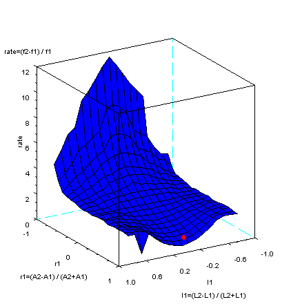
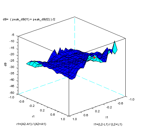
ここでは、2管の全長を17cm、断面積の和を10cm2、一定として、計算している。また、r1は
-0.9から0.9まで0.1ステップで、 l1は -0.8から0.8まで 0.1 ステップで計算している。 参考に、上図を作成するのに使ったSCILABのプログラムをのせておこう。計算には不完全
な部分もある。ファイル名を 2tubemodelmax.sci に変更して使用する。
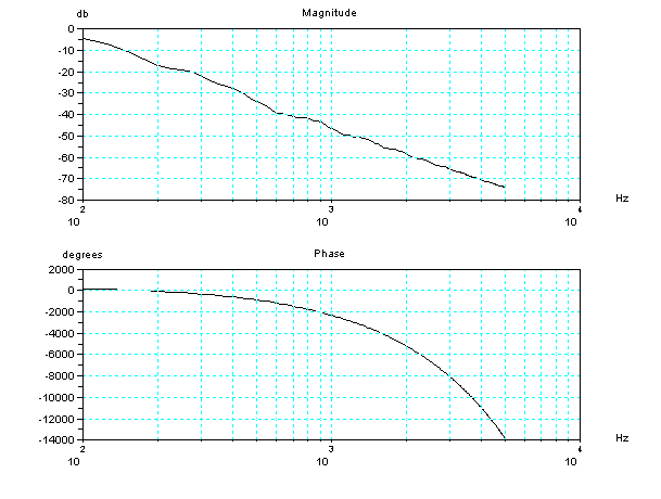
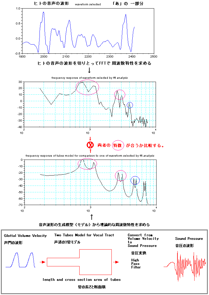
さて、音声波形の生成模型(モデル)の、音声の認識への利用の可能性を考えてみよう。
下の図は、ヒトが話した「あ」の波形の一部分の周波数特性と、音声波形の生成模型(モデル)による周波数特性との比較である。ヒトが話した「あ」に、特徴
が似るように(下図の紫色の丸で囲ったところ)、生成模型(モデル)のパラメータを調整してみた。下の図を見るとわかるとうり、生成模型(モデル)でつ
くった特徴が、実際の音声にも含まれていることがわかる。周波数特性の4KHz以上では、生成模型(モデル)のピークとヒトのピークでは違いがある。ヒト
の口の中の肌は柔らかいので、高い音はそんなに響かないが、生成模型(モデル)は高い周波数の音でも十分に鳴る理想的な管を使っているのでこの違いもひと
つの理由と思われる。
調整は、
生成模型(モデル)のパラメーターの調整値の例
管の全長(L1+L2) 18.5cm
l1=0
r1=0.8
音圧変換用のハイパスフィルターのカットオフfc 1000Hz
声門波形の trise=6ms と tfall=0.7ms
「あ」なので、l1は理想値である0を初期値とする。
管の全長(L1+L2)を変化させることで、ピーク周波数の絶対値を調整する。
1に近い方がよいr1(またはl1)を調整することで、二つの山のピークの周波数の差(ratio)を調整する。
音圧変換用のハイパスフィルターと、声門波形のパラメーターは、周波数特性のエンベロープのカーブの傾斜にも関係するもので、ここでは、合わせこんでいな
い。
ヒトの音声波形と、音声波形の生成模型(モデル)を比較することにより、パラメーターの種類として、
(1)個人で差があるパラメーター 管の全長(L1+L2)。管の全長は物理的な解釈では声門から口(唇)までの長さに相当するが、この解釈は正確では
ない。
(2)音韻に関連するパラメーター l1、r1
(3)音の伝送系に関連するパラメーター fc
(4)その他 trise, tfall
が推定できる。
もしも、「あ」とか「う」などの音韻を成す原理を知っていれば、認識が可能となるであろう。その判別方法は、数値演算だけでなく、ピーク検出や構成を判別
するための、論理演算になるであろう。
参考に、上の周波数特性の比較の図を作ったSCILABのプログラムをデモンストレーション用としてリ
ンクしておきます。
もう一つの例として、「え」を見てみよう。
下の図は、ヒトが話した「え」の波形の一部分の周波数特性と、2管による音声波形の生成模型(モデル)による周波数特性との比較である。上図の「あ」とち
がって「え」は、周波数が低い方の山は一つであるが、高い周波数で山々が、”近
接するように”、たっているのがミソのようだ。このようになるr1とl1の解は、2管による模型では、下図の左右に示すように2種類ある。
物理的に解釈すると、下図の左側は、舌を口の奥でまげていることに相当し、右側は、舌を手前でまげていることに相当する。「あ」の舌のまげ位置が、丁度真
ん中に相当するので、「あ」に対して後方と前方の2種類となる。
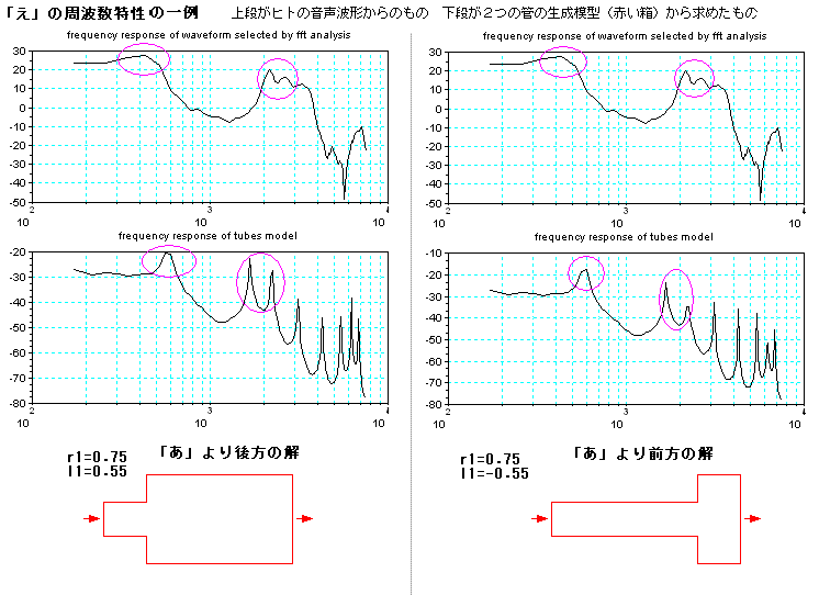
最後に、どこが「え」に聞こえるの?と疑問に思われるかもしれないが、参考に、2管模型で作った2つの波形(後方の解.wav と 前方の解.wav)
をリンクしておこう。
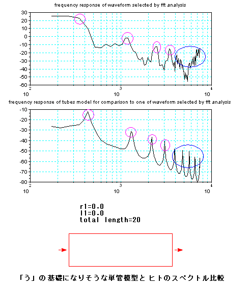
余談であるが、「う」は「あ」とか「え」の様な 近接するピークをもつ特徴を作るのではなく、下図の様に、
単に音を伝える伝送管(単管模型)を基礎としてその管が
実際の現場に応じて多少変形したものと解釈できるかもしれない。
そもそも、1倍(基本波)と2倍と3倍の高調波の波形をそれぞれ適当な比でミックス(MIX)すると、「う」の様に聞こえるようになる。よくありがちな波
形である。

|

|
|
|

|
数値演算ライブラリ
SCILAB |
ディレクトリ型
検索エンジン
|
|
|
W3CによるHTMLの
Web文法チェッカー
|
No.41e
2010年2月27日
2015年11月29日
2018年4月14日
2018年11月7日
since
2007.11